The Wright omega function along part of the real axis
In mathematics, the Wright omega function or Wright function,[note 1] denoted ω, is defined in terms of the Lambert W function as:
Uses
One of the main applications of this function is in the resolution of the equation z = ln(z), as the only solution is given by z = e−ω(πi).
y = ω(z) is the unique solution, when for x ≤ −1, of the equation y + ln(y) = z. Except on those two rays, the Wright omega function is continuous, even analytic.
Properties
The Wright omega function satisfies the relation .
It also satisfies the differential equation
wherever ω is analytic (as can be seen by performing separation of variables and recovering the equation ), and as a consequence its integral can be expressed as:
Its Taylor series around the point takes the form :


 z = Re(ω(x + i y))
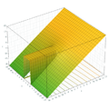 z = Im(ω(x + i y))
 ω(x + i y)


