Capillary wave
Wave on the surface of a fluid, dominated by surface tension


A capillary wave is a wave traveling along the phase boundary of a fluid, whose dynamics and phase velocity are dominated by the effects of surface tension.
Capillary waves are common in nature, and are often referred to as ripples. The wavelength of capillary waves on water is typically less than a few centimeters, with a phase speed in excess of 0.2–0.3 meter/second.
A longer wavelength on a fluid interface will result in gravity–capillary waves which are influenced by both the effects of surface tension and gravity, as well as by fluid inertia. Ordinary gravity waves have a still longer wavelength.
When generated by light wind in open water, a nautical name for them is cat's paw waves. Light breezes which stir up such small ripples are also sometimes referred to as cat's paws. On the open ocean, much larger ocean surface waves (seas and swells) may result from coalescence of smaller wind-caused ripple-waves.
Dispersion relation
The dispersion relation describes the relationship between wavelength and frequency in waves. Distinction can be made between pure capillary waves – fully dominated by the effects of surface tension – and gravity–capillary waves which are also affected by gravity.
Capillary waves, proper
The dispersion relation for capillary waves is

where is the angular frequency, the surface tension, the density of the heavier fluid, the density of the lighter fluid and the wavenumber. The wavelength is For the boundary between fluid and vacuum (free surface), the dispersion relation reduces to


Gravity–capillary waves

![{\displaystyle \scriptstyle {\sqrt[{4}]{g\sigma /\rho }}}](https://wikimedia.org/api/rest_v1/media/math/render/svg/d5fba378198fe7494e9310dfecd81b655747a78c)

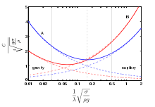
• Blue lines (A): phase velocity, Red lines (B): group velocity.
• Drawn lines: dispersion relation for gravity–capillary waves.
• Dashed lines: dispersion relation for deep-water gravity waves.
• Dash-dotted lines: dispersion relation valid for deep-water capillary waves.
When capillary waves are also affected substantially by gravity, they are called gravity–capillary waves. Their dispersion relation reads, for waves on the interface between two fluids of infinite depth:[1][2]

where is the acceleration due to gravity, and are the mass density of the two fluids . The factor in the first term is the Atwood number.


Gravity wave regime
For large wavelengths (small ), only the first term is relevant and one has gravity waves. In this limit, the waves have a group velocity half the phase velocity: following a single wave's crest in a group one can see the wave appearing at the back of the group, growing and finally disappearing at the front of the group.

Capillary wave regime
Shorter (large ) waves (e.g. 2 mm for the water–air interface), which are proper capillary waves, do the opposite: an individual wave appears at the front of the group, grows when moving towards the group center and finally disappears at the back of the group. Phase velocity is two thirds of group velocity in this limit.
Phase velocity minimum
Between these two limits is a point at which the dispersion caused by gravity cancels out the dispersion due to the capillary effect. At a certain wavelength, the group velocity equals the phase velocity, and there is no dispersion. At precisely this same wavelength, the phase velocity of gravity–capillary waves as a function of wavelength (or wave number) has a minimum. Waves with wavelengths much smaller than this critical wavelength are dominated by surface tension, and much above by gravity. The value of this wavelength and the associated minimum phase speed are:[1]


For the air–water interface, is found to be 1.7 cm (0.67 in), and is 0.23 m/s (0.75 ft/s).[1]
If one drops a small stone or droplet into liquid, the waves then propagate outside an expanding circle of fluid at rest; this circle is a caustic which corresponds to the minimal group velocity.[3]
Derivation
As Richard Feynman put it, "[water waves] that are easily seen by everyone and which are usually used as an example of waves in elementary courses [...] are the worst possible example [...]; they have all the complications that waves can have."[4] The derivation of the general dispersion relation is therefore quite involved.[5]
There are three contributions to the energy, due to gravity, to surface tension, and to hydrodynamics. The first two are potential energies, and responsible for the two terms inside the parenthesis, as is clear from the appearance of and . For gravity, an assumption is made of the density of the fluids being constant (i.e., incompressibility), and likewise (waves are not high enough for gravitation to change appreciably). For surface tension, the deviations from planarity (as measured by derivatives of the surface) are supposed to be small. For common waves both approximations are good enough.
The third contribution involves the kinetic energies of the fluids. It is the most complicated and calls for a hydrodynamic framework. Incompressibility is again involved (which is satisfied if the speed of the waves is much less than the speed of sound in the media), together with the flow being irrotational – the flow is then potential. These are typically also good approximations for common situations.
The resulting equation for the potential (which is Laplace equation) can be solved with the proper boundary conditions. On one hand, the velocity must vanish well below the surface (in the "deep water" case, which is the one we consider, otherwise a more involved result is obtained, see Ocean surface waves.) On the other, its vertical component must match the motion of the surface. This contribution ends up being responsible for the extra outside the parenthesis, which causes all regimes to be dispersive, both at low values of , and high ones (except around the one value at which the two dispersions cancel out.)
| Dispersion relation for gravity–capillary waves on an interface between two semi–infinite fluid domains |
|---|
| Consider two fluid domains, separated by an interface with surface tension. The mean interface position is horizontal. It separates the upper from the lower fluid, both having a different constant mass density, and for the lower and upper domain respectively. The fluid is assumed to be inviscid and incompressible, and the flow is assumed to be irrotational. Then the flows are potential, and the velocity in the lower and upper layer can be obtained from and , respectively. Here and are velocity potentials. Three contributions to the energy are involved: the potential energy due to gravity, the potential energy due to the surface tension and the kinetic energy of the flow. The part due to gravity is the simplest: integrating the potential energy density due to gravity, (or ) from a reference height to the position of the surface, :[6] assuming the mean interface position is at . An increase in area of the surface causes a proportional increase of energy due to surface tension:[7] where the first equality is the area in this (Monge's) representation, and the second applies for small values of the derivatives (surfaces not too rough). The last contribution involves the kinetic energy of the fluid:[8] Use is made of the fluid being incompressible and its flow is irrotational (often, sensible approximations). As a result, both and must satisfy the Laplace equation:[9]
These equations can be solved with the proper boundary conditions: and must vanish well away from the surface (in the "deep water" case, which is the one we consider). Using Green's identity, and assuming the deviations of the surface elevation to be small (so the z–integrations may be approximated by integrating up to instead of ), the kinetic energy can be written as:[8] To find the dispersion relation, it is sufficient to consider a sinusoidal wave on the interface, propagating in the x–direction:[7] with amplitude and wave phase . The kinematic boundary condition at the interface, relating the potentials to the interface motion, is that the vertical velocity components must match the motion of the surface:[7]
To tackle the problem of finding the potentials, one may try separation of variables, when both fields can be expressed as:[7] Then the contributions to the wave energy, horizontally integrated over one wavelength in the x–direction, and over a unit width in the y–direction, become:[7][10] The dispersion relation can now be obtained from the Lagrangian , with the sum of the potential energies by gravity and surface tension :[11] For sinusoidal waves and linear wave theory, the phase–averaged Lagrangian is always of the form , so that variation with respect to the only free parameter, , gives the dispersion relation .[11] In our case is just the expression in the square brackets, so that the dispersion relation is: the same as above. As a result, the average wave energy per unit horizontal area, , is: As usual for linear wave motions, the potential and kinetic energy are equal (equipartition holds): .[12] |


![{\displaystyle V_{\mathrm {st} }=\sigma \iint dx\,dy\;\left[{\sqrt {1+\left({\frac {\partial \eta }{\partial x}}\right)^{2}+\left({\frac {\partial \eta }{\partial y}}\right)^{2}}}-1\right]\approx {\frac {1}{2}}\sigma \iint dx\,dy\;\left[\left({\frac {\partial \eta }{\partial x}}\right)^{2}+\left({\frac {\partial \eta }{\partial y}}\right)^{2}\right],}](https://wikimedia.org/api/rest_v1/media/math/render/svg/4708c19acff7de64c97332d51cc2923b7a48cf00)
![{\displaystyle T={\frac {1}{2}}\iint dx\,dy\;\left[\int _{-\infty }^{\eta }dz\;\rho \,\left|\mathbf {\nabla } \Phi \right|^{2}+\int _{\eta }^{+\infty }dz\;\rho '\,\left|\mathbf {\nabla } \Phi '\right|^{2}\right].}](https://wikimedia.org/api/rest_v1/media/math/render/svg/7a02fa05cd0b2280b73fdb1e4638e92e09f13f7e)


![{\displaystyle T\approx {\frac {1}{2}}\iint dx\,dy\;\left[\rho \,\Phi \,{\frac {\partial \Phi }{\partial z}}\;-\;\rho '\,\Phi '\,{\frac {\partial \Phi '}{\partial z}}\right]_{{\text{at }}z=0}.}](https://wikimedia.org/api/rest_v1/media/math/render/svg/6819b4e24e6b0c3c6746fdb276edde7d22414411)


![{\displaystyle L={\frac {1}{4}}\left[(\rho +\rho '){\frac {\omega ^{2}}{|k|}}-(\rho -\rho ')g-\sigma k^{2}\right]a^{2}\lambda .}](https://wikimedia.org/api/rest_v1/media/math/render/svg/b98c5da92c6d3474ee71b2a4f60dd9c2c8210b1f)


![{\displaystyle {\bar {E}}={\frac {1}{2}}\,\left[(\rho -\rho ')\,g+\sigma k^{2}\right]\,a^{2}.}](https://wikimedia.org/api/rest_v1/media/math/render/svg/ca523bb7fe7083ef2fe607f96709f4d0bada97db)

See also
- Capillary action
- Dispersion (water waves)
- Fluid pipe
- Ocean surface wave
- Thermal capillary wave
- Two-phase flow
- Wave-formed ripple
Gallery
-
 Ripples on water created by water striders
 -
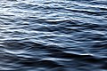 Light breeze ripples in the surface water of a lake


Notes
- ^ a b c Lamb (1994), §267, page 458–460.
- ^ Dingemans (1997), Section 2.1.1, p. 45.
Phillips (1977), Section 3.2, p. 37. - ^ Falkovich, G. (2011). Fluid Mechanics, a short course for physicists. Cambridge University Press. Section 3.1 and Exercise 3.3. ISBN 978-1-107-00575-4.
- ^ R.P. Feynman, R.B. Leighton, and M. Sands (1963). The Feynman Lectures on Physics. Addison-Wesley. Volume I, Chapter 51-4.
- ^ See e.g. Safran (1994) for a more detailed description.
- ^ Lamb (1994), §174 and §230.
- ^ a b c d e Lamb (1994), §266.
- ^ a b Lamb (1994), §61.
- ^ Lamb (1994), §20
- ^ Lamb (1994), §230.
- ^ a b Whitham, G. B. (1974). Linear and nonlinear waves. Wiley-Interscience. ISBN 0-471-94090-9. See section 11.7.
- ^ Lord Rayleigh (J. W. Strutt) (1877). "On progressive waves". Proceedings of the London Mathematical Society. 9: 21–26. doi:10.1112/plms/s1-9.1.21. Reprinted as Appendix in: Theory of Sound 1, MacMillan, 2nd revised edition, 1894.
References
- Longuet-Higgins, M. S. (1963). "The generation of capillary waves by steep gravity waves". Journal of Fluid Mechanics. 16 (1): 138–159. Bibcode:1963JFM....16..138L. doi:10.1017/S0022112063000641. ISSN 1469-7645. S2CID 119740891.
- Lamb, H. (1994). Hydrodynamics (6th ed.). Cambridge University Press. ISBN 978-0-521-45868-9.
- Phillips, O. M. (1977). The dynamics of the upper ocean (2nd ed.). Cambridge University Press. ISBN 0-521-29801-6.
- Dingemans, M. W. (1997). Water wave propagation over uneven bottoms. Advanced Series on Ocean Engineering. Vol. 13. World Scientific, Singapore. pp. 2 Parts, 967 pages. ISBN 981-02-0427-2.
- Safran, Samuel (1994). Statistical thermodynamics of surfaces, interfaces, and membranes. Addison-Wesley.
- Tufillaro, N. B.; Ramshankar, R.; Gollub, J. P. (1989). "Order-disorder transition in capillary ripples". Physical Review Letters. 62 (4): 422–425. Bibcode:1989PhRvL..62..422T. doi:10.1103/PhysRevLett.62.422. PMID 10040229.
External links
Wikimedia Commons has media related to Ripples (water waves).
- Capillary waves entry at sklogwiki
| Authority control databases: National |
|
|---|


